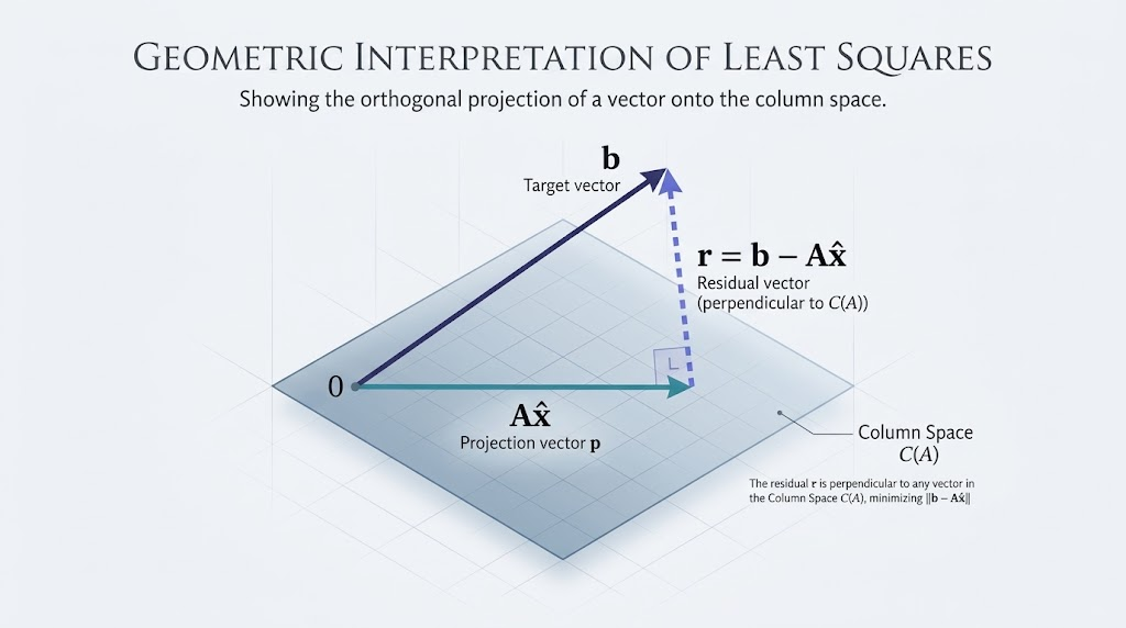
Least squares

Updated 03 Nov 2026

•
Objective
- •
  choose $x$ to minimize $\lVert Ax-b\rVert_2^2$ for an overdetermined or inconsistent system.
- •
  Normal equations -> a minimizer satisfies the normal equations $A^\mathsf{T}A\hat{x}=A^\mathsf{T}b$ .
- •
  Full column rank $\hat{x}=(A^\mathsf{T}A)^{-1}A^\mathsf{T}b$ .
- •
  Geometry
  - •
    Projection -> $A\hat x$ projects $b$ onto the column space of $A$ .
  - •
    Orthogonality -> $A^T(b-A\hat x)=0$ ; the residual is perpendicular to that space.
- •
- •
•
Numerical pratice
- •
  the inverse expression is not the preferred computational procedure.
- •
  forming $A^\mathsf{T}A$ squares the 2-norm condition number: $\kappa_2(A^TA)=\kappa_2(A)^2$ for full column rank.
- •
  QR or SVD is often more reliable, especially when columns are nearly dependent.
  - •
    Thin QR -> $A=QR$ , with orthonormal columns in $Q$ ; solve $R\hat x=Q^Tb$ .
  - •
    center/scale polynomial predictors to reduce avoidable numerical scaling problems.
- •
  Dependent columns
  - •
    the inverse may not exist; minimizers may not be unique.
  - •
    SVD can produce a minimum-norm solution.
•
Uses and worked line fit
- •
  overdetermined systems connect with regression and curve fitting
- •
  Regression models
  - •
    Simple -> $\hat y=\beta_0+\beta_1x$ .
  - •
    Multiple -> $\hat y=\beta_0+\sum_j\beta_jx_j$ .
  - •
    linear means linear in coefficients; supplied features may include $x^2$ .
- •
  Centered simple fit
  - •
    Slope -> $\beta_1=\sum_i(x_i-\bar x)(y_i-\bar y)/\sum_i(x_i-\bar x)^2$ .
  - •
    Intercept -> $\beta_0=\bar y-\beta_1\bar x$ .
  - •
    avoids explicitly forming/inverting $A^TA$ for a two-parameter line.
- •
  Example
  - •
    data: $x=(1,2,3,4,5)$ , $y=(2,3,5,6,8)$ .
  - •
    Fitted line -> $\hat y=0.3+1.5x$ .
  - •
    at $x=6$ , $\hat y=9.3$ .
  - •
    Training SSE -> $0.3$ .
  - •
    Training RMSE -> $\sqrt{0.3/5}\approx0.244949$ .
  - •
    coefficients 15 and 3/prediction 93 do not fit these observations.
- •
  Excel functions
  - •
    Intercept -> INTERCEPT, not INTERSECT.
  - •
    Forecast -> FORECAST.LINEAR(new_x, known_y, known_x) separates query and training data.
- •
  Interpretation
  - •
    Interpolation vs fitting -> Interpolation forces a fit through nodes; least squares generally allows residuals.
  - •
    use unseen data.
  - •
    fitting does not establish causation.
•
Model construction
- •
  Simple-line normal equations
  - •
    $n\beta_0+\beta_1\sum_i x_i=\sum_i y_i$ .
  - •
    $\beta_0\sum_i x_i+\beta_1\sum_i x_i^2=\sum_i x_i y_i$ .
  - •
    obtain them by setting the SSE derivatives with respect to both coefficients to zero.
- •
  Through-origin fit
  - •
    if a zero intercept is physically justified, use $\hat y=\beta_1x$ .
  - •
    $\beta_1=\sum_i x_i y_i/\sum_i x_i^2$ , provided the denominator is positive.
  - •
    this is a different constraint, not a substitute for estimating an intercept.
- •
  Polynomial fit
  - •
    degree $m$ : $\hat y=\sum_{j=0}^m a_jx^j$ ; design matrix $X_{ij}=x_i^j$ .
  - •
    still linear in the coefficients, although curved as a function of $x$ .
  - •
    increasing degree can reduce training SSE while worsening generalization and conditioning.
  - •
    there is no universal degree at which every polynomial fit becomes unstable.
- •
  Multiple predictors
  - •
    use columns $[1,x_1,\ldots,x_p]$ for an intercept and $p$ predictors.
  - •
    a quadratic two-variable response surface uses $[1,x_1,x_2,x_1x_2,x_1^2,x_2^2]$ .
  - •
    coefficients describe conditional associations; a fitted coefficient alone is not a causal effect.
- •
  Multicollinearity
  - •
    near-dependent predictor columns make individual coefficient estimates sensitive.
  - •
    Variance inflation factor -> $\mathrm{VIF}_j=1/(1-R_j^2)$ .
  - •
    here $R_j^2$ comes from regressing predictor $j$ on the other predictors, with an intercept.
  - •
    with only two predictors, $R_j^2$ is their squared correlation.
  - •
    cutoffs such as VIF 10 are heuristics, not guarantees of model quality.
•
Linearizing nonlinear models
- •
  Exponential -> $y=\alpha e^{\beta x}$ .
  - •
    fit $\ln y=a_0+a_1x$ ; recover $\alpha=e^{a_0}$ and $\beta=a_1$ .
  - •
    requires $y>0$ .
- •
  Power law -> $y=\alpha x^\beta$ .
  - •
    fit $\log y=a_0+a_1\log x$ using one consistent log base.
  - •
    with natural logs, $\alpha=e^{a_0}$ and $\beta=a_1$ ; requires $x,y>0$ .
- •
  Saturation / Michaelis-Menten -> $y=\alpha x/(\beta+x)$ .
  - •
    fit $1/y=a_0+a_1/x$ ; recover $\alpha=1/a_0$ , $\beta=a_1/a_0$ .
  - •
    requires nonzero transformation arguments and a valid recovered model domain.
- •
  The loss changes
  - •
    least squares after transformation minimizes transformed residuals, not original-scale SSE.
  - •
    for small additive errors, log-space fitting approximately weights original squared residuals by $1/y^2$ .
  - •
    reciprocal-space fitting approximately weights them by $1/y^4$ .
  - •
    choose according to the error model; transformed fitting is not inherently wrong or always inferior.
  - •
    a transformed fit can provide initial values for original-scale nonlinear least squares with scipy.optimize.curve_fit.
- •
  Engineering models
  - •
    Decay -> $N(t)=N_0e^{-\lambda t}$ ; half-life $T_{1/2}=\ln2/\lambda$ for $\lambda > 0$
  - •
    Arrhenius -> $k(T)=A e^{-E_a/(RT)}$ ; $\ln k=\ln A-(E_a/R)(1/T)$ .
  - •
    use absolute temperature and compatible energy units; a slope in $1/T$ determines $-E_a/R$ .
•
Fit quality and residual diagnostics
- •
  define $e_i=y_i-\hat y_i$ ; $S_r=\sum_i e_i^2$ , $S_t=\sum_i(y_i-\bar y)^2$ .
- •
  let $q$ be the number of fitted coefficients, including an intercept; require $n>q$ for residual degrees of freedom
- •
  Metrics
  - •
    RMSE -> $\sqrt{S_r/n}$ ; error scale in response units
  - •
    MAE -> $\sum_i|e_i|/n$ ; less dominated by large errors than squared loss
  - •
    Residual standard deviation -> $s=\sqrt{S_r/(n-q)}$ ; not the same denominator as RMSE.
  - •
    Determination -> $R^2=1-S_r/S_t$ , for $S_t>0$ .
  - •
    Adjusted determination -> $R_{\mathrm{adj}}^2=1-[S_r/(n-q)]/[S_t/(n-1)]$ .
  - •
    $R^2$ can be negative, especially on held-out data; the formula is undefined for constant targets.
  - •
    adding regressors need not imrpove adjusted $R^2$ ; neither metric alone proves generalization
- •
  Residual plots
  - •
    curvature -> possible missing model structure
  - •
    funnel-shaped spread -> possible nonconstant variance; consider an appropriate model or weighted least squares
  - •
    patterns over time/order -> possible dependence; appearance alone does not prove independence
  - •
    squared loss is outlier-sensitive; investigate unusual data and consider justified robust losses such as absolute or Huber loss
- •
  Additional diagnostics
  - •
    Durbin-Watson -> $d=\sum_{i=2}^n(e_i-e_{i-1})^2/\sum_i e_i^2$ .
    
    •
    values near 2 suggest little first-order residual autocorrelation; formal interpretation requries suitable assumptions
  - •
    Overall F statistic -> $F=[R^2/p]/[(1-R^2)/(n-p-1)]$ for $p$ predictors plus an intercept
    
    •
    tests the joint slope restriction under the regression assumptions; not a measure of causal impact
  - •
    AIC -> $n\ln(S_r/n)+2k$ , up to shared constants for a Gaussian-error likelihood with estimated variance
    
    •
    count all fitted likelihood parameters consistently: $k=q+1$ when variance is estimated too
    
    •
    compare compatible likelihoods on the same observations/response scale;
- •
  compare models using held-out evidence as well as in-sample diagnostics; see evaluation splits and leakage
•
Worked comparisons
- •
  Sensor/strain line
  - •
    $x=(1,2,3,4,5)$ , $y=(70,142,208,282,350)$ -> $\hat y=0.4+70x$ .
  - •
    with $x$ in $10^{-3}$ strain and $y$ in MPa, the slope corresponds to an elastic modulus of 70 GPa.
  - •
    $S_r=11.2$ , $R^2\approx0.99977148$ .
  - •
    replacing only the last $y$ with 500 gives $\hat y=-59.6+100x$ .
  - •
    a single outlier can strongly move a squared-loss fit.
- •
  Quadratic fit
  - •
    $x=(0,1,2,3,4)$ , $y=(1,1.8,1.3,2.5,6.3)$ .
  - •
    $\hat y=1.42-1.07x+0.55x^2$ .
- •
  Adjusted- $R^2$ comparison
  - •
    for $n=6$ , $S_t=100$ : a line with $S_r=15$ gives $R^2=0.85$ , adjusted $R^2=0.8125$ .
  - •
    a quartic with $S_r=10$ gives $R^2=0.90$ , adjusted $R^2=0.50$ .
  - •
    lower training SSE is not automatically a better-supported model.
- •
  Multiple-regression correction
  - •
    data $(x_1,x_2,y)$ : $(20,25,150),(40,25,210),(60,30,290),(80,30,350)$ .
  - •
    the fitted model is $\hat y=-10+3x_1+4x_2$ , not the PDF's printed coefficients.

Python: array-based curve fitting

•
standalone block using NumPy and SciPy; original-scale residuals are compared on the same observations.
•
lstsq avoids an explicit normal-equation inverse; polynomial columns are ordered constant, linear, quadratic.
•
curve_fit covariance is an approximate uncertainty estimate under assumptions, not automatic confidence intervals.

import numpy as np
from scipy.optimize import curve_fit

x = np.array([0., 1., 2., 3., 4.])
y = np.array([1., 1.8, 1.3, 2.5, 6.3])
X = np.column_stack((np.ones_like(x), x, x*x))
coefficients, _, rank, _ = np.linalg.lstsq(X, y, rcond=None)
assert rank == X.shape[1]
assert np.allclose(coefficients, [1.42, -1.07, 0.55])

substrate = np.array([1., 2., 5., 10.])
rate = np.array([2.5, 4., 6.3, 7.7])
Z = np.column_stack((np.ones_like(substrate), 1/substrate))
a0, a1 = np.linalg.lstsq(Z, 1/rate, rcond=None)[0]
initial = np.array([1/a0, a1/a0])
def saturation(s, vmax, km):
      return vmax*s/(km+s)
fitted, covariance = curve_fit(saturation, substrate, rate, p0=initial, bounds=(0, np.inf))
def rmse(parameters):
      return np.sqrt(np.mean((rate - saturation(substrate, *parameters))**2))
assert rmse(fitted) <= rmse(initial)
assert np.allclose(initial, [10.06879170, 3.028094885], rtol=1e-7)
print("quadratic coefficients:", coefficients)
print("reciprocal fit:", initial, "original-scale RMSE:", rmse(initial))
print("nonlinear fit:", fitted, "original-scale RMSE:", rmse(fitted))

•

Python: centered least squares

•
numerically stable centered linear regression in Python
- •
  the algorithm is a finite two-parameter closed-form fit; no iteration cap needed
- •
  spread_tol rejects near-constant predictors
- •
  use QR/SVD for multiple columns, for example numpu.linalg.lstsq

•

import math

def fit_line(xs, ys, spread_tol=1e-12):
      xs, ys = list(xs), list(ys)
      if len(xs) != len(ys) or len(xs) < 2:
          raise ValueError("need equal lengths and at least two observations")
      if not math.isfinite(spread_tol) or spread_tol <= 0:
          raise ValueError("positive finite spread tolerance required")
      if not all(math.isfinite(v) for v in xs+ys):
          raise ValueError("nonfinite data")
      n = len(xs)
      mx, my = math.fsum(v/n for v in xs), math.fsum(v/n for v in ys)
      dx = [v-mx for v in xs]
      scale = max(1.0, max(abs(v) for v in xs))
      spread = max(abs(v) for v in dx)
      if not math.isfinite(spread) or spread/scale <= spread_tol:
          raise ValueError("predictors constant or numerically unresolved")
      ux = [v/spread for v in dx]
      scaled_slope = math.fsum(u*(y-my) for u, y in zip(ux, ys))/math.fsum(u*u for u in ux)
      slope = scaled_slope/spread
      intercept = my-slope*mx
      residuals = [y-(intercept+slope*x) for x, y in zip(xs, ys)]
      sse = math.fsum(r*r for r in residuals)
      if not all(math.isfinite(v) for v in (slope, intercept, sse)):
          raise ValueError("fit overflow or nonfinite result")
      return intercept, slope, sse, math.sqrt(sse/n)

intercept, slope, sse, rmse = fit_line([1,2,3,4,5], [2,3,5,6,8])
assert math.isclose(intercept, 0.3, abs_tol=1e-14)
assert math.isclose(slope, 1.5, abs_tol=1e-14)
assert math.isclose(sse, 0.3, abs_tol=1e-14)
assert math.isclose(intercept+6*slope, 9.3, abs_tol=1e-14)
for xs, ys in [([1,1], [2,3]), ([1,2], [3]), ([1,math.nan], [2,3])]:
      try:
          fit_line(xs, ys)
      except ValueError:
          pass
      else:
          raise AssertionError("invalid fit accepted")
print(f"least squares: intercept={intercept:.12f}, slope={slope:.12f}, "
        f"prediction(6)={intercept+6*slope:.12f}, SSE={sse:.12f}, RMSE={rmse:.12f}")

•

Excel VBA: centered least squares

•
numerically stable centered linear regression in Excel VBA; no explicit matrix inverse
- •
  input checks: equal one-column numeric ranges, at least two rows, sufficient relative predictor spread
- •
  VBA errors fro invalid cells, rank failure, or arithmetic overflow
•
Setup and calls
1. 1.
  put $1,2,3,4,5$ in A2:A6 on the active worksheet
2. 2.
  put $2,3,5,6,8$ in B2:B6
3. 3.
  run DemoLeastSquares; it doesn't write cells
- •
  return value: intercept, slope, SSE, RMSE
- •
  Worksheet comparisons
  - •
    slope: =SLOPE(B2:B6,A2:A6).
  - •
    intercept: =INTERCEPT(B2:B6,A2:A6).
  - •
    prediction at 6: =FORECAST.LINEAR(6,B2:B6,A2:A6).
- •
  an iteration count is not applicable to this direct finite fit
- •
  spreadTol is a numerical rank threshold, not a residual target

•

Private Function FitCell(ByVal cell As Range) As Double
      Dim value As Variant
      value = cell.Value2
      If IsError(value) Then Err.Raise vbObjectError + 401, "FitLine", "Error cell"
      If IsEmpty(value) Then Err.Raise vbObjectError + 402, "FitLine", "Empty cell"
      If VarType(value) = vbBoolean Or VarType(value) = vbString Then _
          Err.Raise vbObjectError + 403, "FitLine", "Numeric cells required"
      If Not IsNumeric(value) Then Err.Raise vbObjectError + 404, "FitLine", "Nonnumeric cell"
      FitCell = CDbl(value)
  End Function

  Public Function FitLine(ByVal xs As Range, ByVal ys As Range, _
      Optional ByVal spreadTol As Double = 0.000000000001) As Variant
      Dim n As Long, i As Long, mx As Double, my As Double
      Dim spread As Double, scale As Double, dx As Double, ux As Double
      Dim sxx As Double, sxy As Double, slope As Double, intercept As Double
      Dim residual As Double, sse As Double, x() As Double, y() As Double
      If xs.Areas.Count <> 1 Or ys.Areas.Count <> 1 Or xs.Columns.Count <> 1 Or ys.Columns.Count <> 1 Then _
          Err.Raise vbObjectError + 405, "FitLine", "Single contiguous columns required"
      n = xs.Rows.Count
      If n < 2 Or n <> ys.Rows.Count Or spreadTol <= 0# Then _
          Err.Raise vbObjectError + 406, "FitLine", "Invalid dimensions or spread tolerance"
      ReDim x(1 To n): ReDim y(1 To n): scale = 1#
      For i = 1 To n
          x(i) = FitCell(xs.Cells(i, 1)): y(i) = FitCell(ys.Cells(i, 1))
          mx = mx + x(i) / n: my = my + y(i) / n
          If Abs(x(i)) > scale Then scale = Abs(x(i))
      Next i
      For i = 1 To n
          dx = Abs(x(i) - mx): If dx > spread Then spread = dx
      Next i
      If spread / scale <= spreadTol Then _
          Err.Raise vbObjectError + 407, "FitLine", "Predictors constant or unresolved"
      For i = 1 To n
          ux = (x(i) - mx) / spread
          sxx = sxx + ux * ux: sxy = sxy + ux * (y(i) - my)
      Next i
      slope = (sxy / sxx) / spread: intercept = my - slope * mx
      For i = 1 To n
          residual = y(i) - (intercept + slope * x(i))
          sse = sse + residual * residual
      Next i
      FitLine = Array(intercept, slope, sse, Sqr(sse / n))
  End Function

  Public Sub DemoLeastSquares()
      Dim result As Variant, ws As Worksheet
      On Error GoTo Failed
      Set ws = ActiveSheet
      result = FitLine(ws.Range("A2:A6"), ws.Range("B2:B6"))
      Debug.Print "intercept", result(0), "slope", result(1)
      Debug.Print "SSE", result(2), "RMSE", result(3)
      Debug.Print "prediction x=6", result(0) + 6# * result(1)
      Exit Sub
  Failed:
      Debug.Print "FAILED: " & Err.Description
  End Sub

Linked references 1

numerical-methods-polban

◌ Explore connections in Graph view

Least squares

Objective

Numerical pratice

Uses and worked line fit

Model construction

Linearizing nonlinear models

Fit quality and residual diagnostics

Worked comparisons

Python: array-based curve fitting

Python: centered least squares

Excel VBA: centered least squares

Linked references 1